This semester for Columbia’s STCS6701: Probabilistic Models and Machine Learning taught by David Blei, I read a variety of papers on probabilistic machine learning. Below I include some short write ups on my thoughts for some of the papers, organized by topics.
Bayesian Inspired Regularizers for Neural Nets
Curvature-Driven Smoothing: A Learning Algorithm for Feedforward Networks, Bayesian Back-Propagation (Section 5)
These two papers explored different priors that could be used with Neural Nets. The first paper, focused on creating a functional smoothness prior based on the second derivative of a neural net with respect to the input. This prior is added to the traditional MSE loss function, thus the learning algorithm will penalize neural nets with large “curvatures” or changes in magnitudes, thus potentially learning a smoother function. The second paper focuses on smoothing priors and entropic priors (priors that nudge the model away from being very confident in a single estimate).
Having mostly focused on lasso and ridge regularization in machine learning, I found reading about these different priors exciting. After reading these papers, what was not fully clear to me was the effectiveness of these priors. My impression was that both priors should be used with smaller sample sizes to avoid overfitting to little data. However, this is also true with lasso / ridge, so it was not clear when to use these priors. The second paper provides a figure showing their proposed smoothness regularizer creates smoother outputs than ridge regularization. Further, they suggest that because of a lack of smooth outputs, ridge regularization overfits based on smaller cluster of points. However, it has been shown that neural nets trained on modern learning algorithms are biased towards smoother (low frequency) functions, so it could be the case that the smoothing prior is redundant. Either way, further empirical tests to understand the efficacy of these priors. Another interesting question is how a model would perform when combining these priors (i.e the prior is that the function should be smooth, and the parameters have mean 0). However, one concern I have (in particular with the smoothing priors) is the computation cost of running it. The first paper mentions their efficient learning algorithm works best with smaller number of inputs. This might be problematic in modern deep learning settings, where input sizes (both in number and dimension) are massive. It could be the case where some of these priors do provide some benefit, however the computation costs outweighs the benefit vs common regularization techniques.
Handling Sparsity via the Horseshoe
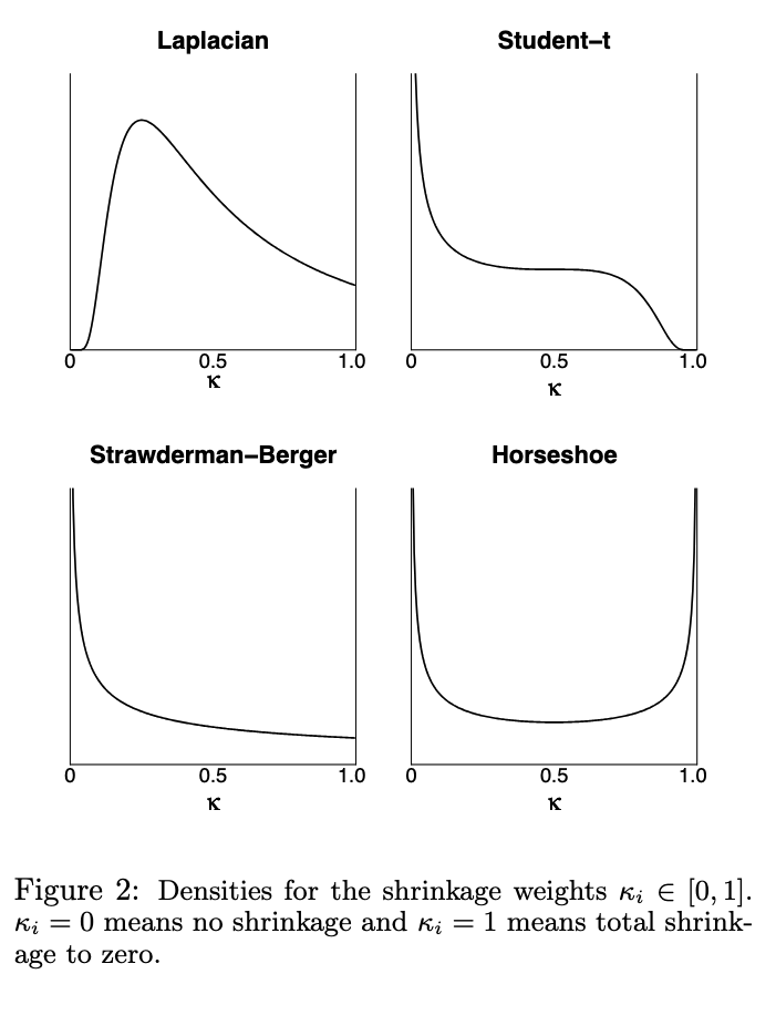
This paper proposed the Horseshoe prior, for learning sparse parameterizations. The authors demonstrate that horseshoe prior, which assume each parameter can be parametrized as $\beta_i \sim N(0, \lambda_i^2 \tau^2)$, where both $\lambda, \tau$ are sampled from a half cauchy distribution, produces sparer parameter estimates (i.e The parameters have a high density at 0 or 1 and a lower density for all other values) than other comparable priors such as the student-t prior or Laplacian prior. In particular, I found Figure 2 of the page (Figure below) very insightful for the efficacy of the Horseshoe prior.
The end result of using a horseshoe prior could have several important benefits for training neural nets. For example, truly sparse parameters could result in a neural net that is easier to interpret, not over parametrized (since extra parameters would have value 0), and is more likely to generalize (since it is not overparameterized). At the same time, I’m not sure how simple it would be to implement the horseshoe prior with a neural net. For example, sampling from a half-Cauchy distribution for thousands of parameters could be time and memory-intensive. Further, I wonder if the heavy tails of the half cauchy distribution as well as the infinite spike at zero would cause problems for modern optimizers with exploding / vanishing gradients.
Variational Dropout Sparsifies Deep Neural Networks
This paper explores how to train Neural Nets with Variational Dropout - an automatic relevance determination (ARD) method. The goal is to learn which parameters of a neural net can be dropped to create a sparser network. The authors do this by initializing a neural net where each weight $w_i \sim \mathcal{N}(\theta_i, \alpha_i)$ where $\theta, \alpha$ are learned parameters. Previous papers used a similar framework, however had difficulties training for large values of $\alpha_i > 1$ given large gradient variance under the prior framework. To overcome this, the authors propose a new method to construct the weights $w_i$ such that the weight’s derivatives have less variance for different $\alpha_i$. Given these new weights, they approximate a function to estimate the KL divergence, which is used as a regularizer in the objective function. The authors proceed to demonstrate their method is able to gain comparable accuracy to Neural Nets that do not use this method, but with much higher levels of sparsity (40-60x more sparsity for some datasets).
Overall, I though the results of the paper were impressive. My overall remaining question for the paper is why these results matter. The increased sparsity does not lead to increased accuracy (and in some cases, slightly less accuracy), which to me was a bit surprising given I’d assume that a sparse network learns less of the training data noise, and hence can generalize better. The authors do briefly comment on that their method can avoid “memorizing” the data, but provide little supporting evidence. The authors tested their methods on the MNIST / CIFAR datasets, which are smaller and simpler classification tasks, which may be the reason why its harder to see if the model trained in variational dropout performs better.
Matrix Factorization
Modeling User Exposure in Recommendation
This paper focused on methods for using matrix factorization models with implicit data. A common challenge with implicit data is the recommendation system may not know if a user did not interact with an item because they didn’t like it or they were not exposed to it. This paper looks to overcome this issue by estimating an extra latent variable $a_{ij}$, which indicates whether or not a user was exposed to the item. If no, the user-item combination is not used when estimating the log joint probability model. To estimate $a_{ij}$, the authors look at two potential measures - 1) how popular an item is - the more popular an item, the more likely a user has seen it and 2) other available factors that might make an item more or less likely to interact with it (for example, a systems researcher is more likely to be exposed to systems papers than machine learning papers).
I generally thought the idea of the paper was interesting and the proposed model for incorporating exposure of an item made sense. Unobserved confounding variables play a large role (especially in implicit / passive observation data) in why a certain user chose a certain item, so adjusting for them is beneficial to creating better recommendations. To demonstrate the performance improvement, the paper provides comparison in different recommendation datasets between WMF (state of the art method at the moment) and ExpoMF (method from the paper). ExpoMF exhibited slightly better performance on 3 of the 4 datasets, which could be interpreted as the method better estimates item exposure. However, without having a source of truth dataset (of which items a user was exposed to), it is difficult to determine the efficacy of the two methods proposed to estimate $u_{ij}$. An interesting final observation is that the paper’s method to adjust for popularity is equivalent to using Manski’s natural bounds, thus giving theoretical justification for the method.
Scalable Recommendation with Poisson Factorization
The paper I read this week proposes a hierarchical Poisson matrix factorization (HPF) and a corresponding variation inference method that is optimized for sparsely populated matrices. The hierarchical portion comes from the adjustment to a normal Poisson factorization where extra latent variables are estimated to adjust for a user’s consumption activity and an item’s popularity. I had a few observations and thoughts. First, I noticed that both this paper and the Expo MF paper used implicit data, but truncated the data to be either 0 or 1. In both cases I was not sure what was the benefit of doing so. Presumably, truncating the data to be either 0 or 1 makes the data cleaner since values of $\geq 1$ are likely rarer and may cause more noise, however, intuitively, there should be useful data in the number of times a user consumed something (more times means a higher preference). Second, I found Figure 6 - a breakdown of articles grouped by different components of $\beta$) - interesting. An interesting extension could potentially be to run the same analysis, but to have a language model interpret each component, thus creating a simple, yet automated explanation system (i.e you read a lot of articles with planes, therefore we recommended this article on planes). Finally, with matrix factorization model, the latent attribute and preferences variables capture the influence of several unobserved variables. However, in many of these datasets, some of these variables could be observed (e.g. movie genre, director, cover art, etc). Given these features, another potential route to further explain how recommendations are created would be to map observed feature vectors to the corresponding preference / attributes latent variables, and measure how much of the variance of the latent variables is captured by the observed feature vectors.
Causal Inference
The Blessings of Multiple Causes
The paper I read this week focused on methods to adjust for unobserved confounding bias when trying to measure the effect of multiple causes on a outcome variable. The main idea is to 1) fit a factor model to capture the joint distribution of the causes and estimate latent variable $Z_i$, 2) estimate $z_i = E[Z_i | A_i = a]$ and 3) condition on $z_i$ when using $A_i$ to predict the outcome variable, $Y$ (i.e. estimate $E[Y_{i}(a) | z)_i, A_i = a]$. Through this method, one could estimate the potential confounding bias between all the causes, and block the backdoor path from $a_i \leftarrow z_i \rightarrow y_i$, thus removing the bias caused from the confounding variables when estimating the effect of the causes on the outcome variable.
I initially read the paper to see if the deconfounder method could adjust for confounding bias in recommender system. What is interesting about this paper is that it highlights why adjusting for confounding bias in matrix factorization recommender systems is difficult - the matrix factorization captures all confounding bias. In other words, the output latent attributes and preferences vectors both contain causal information (i.e. user xyz enjoys actions movies and therefore will enjoy Indiana Jones) and spurious correlation. To separate the two, one could use the following method. Users and Items are not abstract object and have true latent features that describe them. Using available information on each entity (for example, self reported preference information for a user, or item title / description), one could measure how much the provided information about the entity explains the variance of the learned latent entity attributes. A more advanced idea would be to create a structural causal model to identify the direct, indirect, and spurious correlation between the entity information and the learned attributes, as explored in this report on Causal Fairness Analysis.