Ahead of the next international soccer break in early June 2025, I wanted to publish a quick overview of the methodology I use to create international soccer forecasts on this site. If you have any thoughts on the below, I would love to hear from you at mateojuliani at gmail dot com!

Section 1: Intro and Motivation

In November 2023, I came across these betting odds for the World Cup Qualifying match between Brazil and Argentina:

If you are not familiar with decimals odds, the picture shows a sports book offering a 2.3x payout for every 1 dollar bet if Brazil beats Argentina. Similarly, it offered 3.0x for a draw, and 3.4x for an Argentine victory. Converting those odds to probability (in this case it is easy - we can do so by dividing 1 by the odds), we get the following:

• Implied chance of Brazil winning: 41.6%
• Implied chance of the game ending in a tie: 33.3%
• Implied chance of Argentina winning: 29.4%

For a bit more background, at the time (November 2023), the Argentine nation team had continued its form from the World Cup, while the Brazilian national team was going through some of the worst - if not the worst - form I had ever seen them in.

Therefore, seeing Brazil as the favorite seemed mispriced. The probable reason why Brazil was priced at 2.3x was their home advantage. Prior to this game, Brazil had never lost a World Cup Qualifying match at home. However, past performance is not indicative of future performance (although obviously it can be a good indicator), and Argentina went to win the game following an Otamendi header.

More importantly, the mispriced odds suggested that maybe these sports books weren’t that great at pricing international soccer matches relative to domestic soccer matches (although a larger sample is needed than just one match), which motivates the main question - How could we build a simple model to estimate the win / draw / loss rates of international soccer matches?

The rest of this post is structured as follows: Section 2 describes the general methodology behind the odds published on this website, Section 3 analyzes how effective this methodology is vs. actual results, and Section 4 is a catch all section for my remaining thoughts.

Section 2: Model Methodology

To start, we need a method to rank a team’s overall form. A common methodology is using the Elo system to rate teams, although some adjustments are needed vs the base system. To keep things simple, we will use the Elo ratings from eloratings.net, which compiles and updates each international team’s Elo ratings. You can read more about the methodology here, but some of the main deviations from the base Elo system are:

• Ties are worth half of a win
• The bigger the tournament (e.g. World Cup, Euros, etc), the higher K factor used ¹.
• The K factor is also modified for goal difference. The greater goal difference, the higher K factor used.

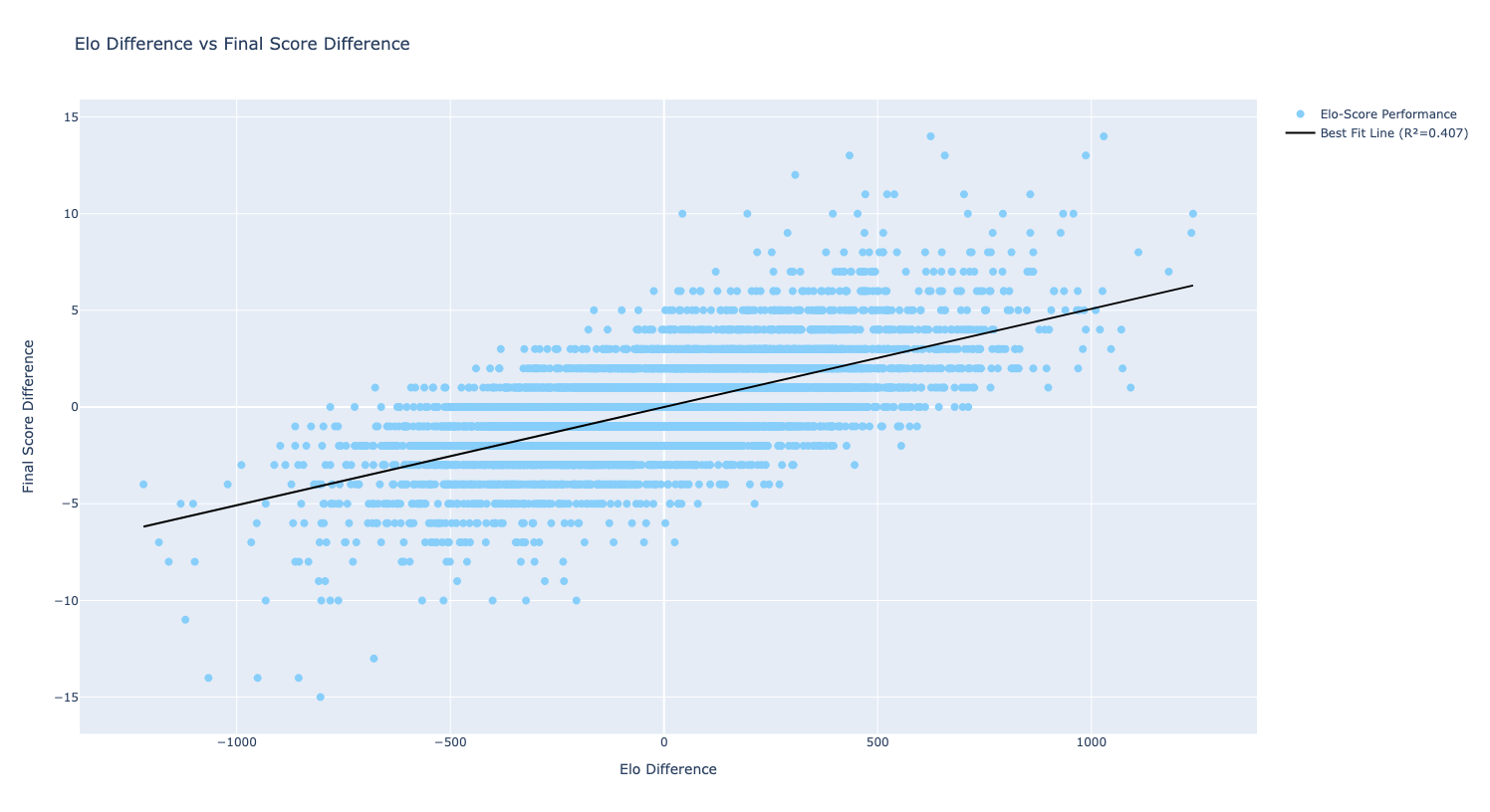
With the Elo ratings, a simple feature we can create to predict win rates is the ELO difference between the two teams. I would highly recommend checking out this video by Oxford Mathematics which details how to use Elo difference to construction a model using Elo difference. In this post, we will use a different methodology, but as shown in the graph below, there is a decent positive relationship (R^2 of ~.41) between ELO difference and score difference.

The Elo difference variable is enough to fit a multinomial logistic regression to forecast win, loss, draw percentages. However, we will add two more features - two dummy variables to indicate if team 1 is home (0 if no, and 1 if yes) and if team 2 is home.

With these three variables, we can fit a multinomial logistic regression using Sklearn. As mentioned, the features are

• elo_diff: The difference in Elo between Team 1 and 2
• team_home: Dummy variable indicating if Team 1 is home
• opp_home: Dummy variable indicating if Team 2 is home

and the target variable is game_results, a category variable indicating if Team 1 won, Team 2 won, or if the game ended in a draw.

X = df_train[["elo_diff", "team_home", "opp_home"]]
y = df_train["game_results"]
model_ft = LogisticRegression(multi_class='multinomial', solver='lbfgs')
model_ft.fit(X, y)

Note, when performing inference, we won’t actually use the model’s direct classification to determine who will win or lose. Instead, we are interested in the probability of each outcome. In other words, we will not use

model_ft.predict()

but instead use to get the probabilities of each of the forecasted classes:

model_ft.predict_proba()

We will then be able to use these probabilities to directly compare to a Sportbook’s odds.

And that is it! Pretty simple, but in the next section will see how well the model performs. If you want to take a closer look at the code, you can find it on my github.

Section 3: Results

Evaluating the results of soccer games is tricky. To start, we will input ELO differences of -1000 to 1000 into our model to get a sense if the model odds are realistic. We also assume that Team 1 is the home team:

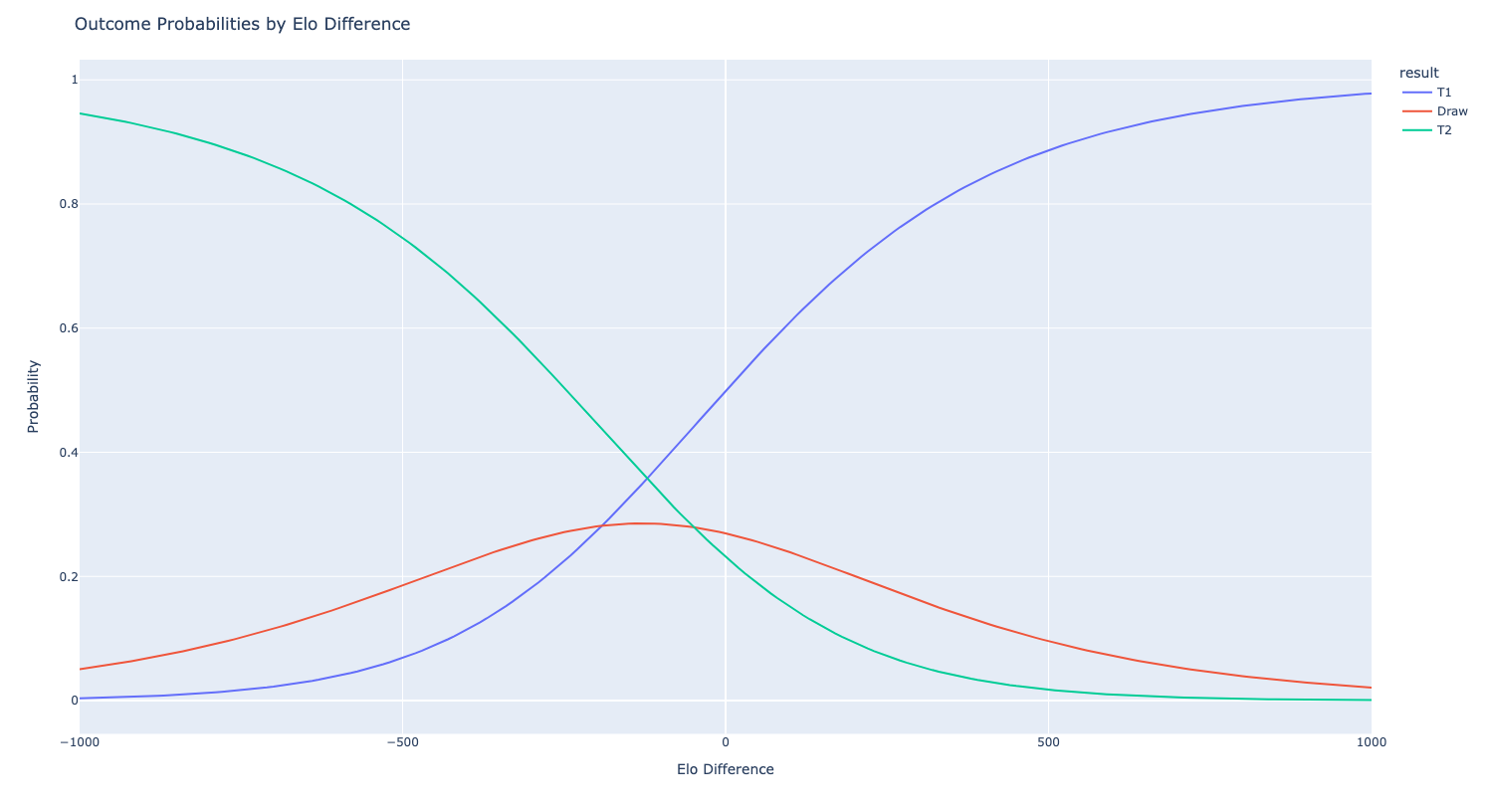
At a high level, we can see as Elo difference increases, Team 1 has higher odds of winning, which is what we would expect. Interestingly, Team 1 and Team 2 have the same odds of winning when Team 1 has an ELO difference of -120 vs Team 2. In other words, the model implies that playing at home is equivalent to getting a 120 point ELO boost. To confirm this, we can plot the same graph but set the home advantage to 0 for both teams.

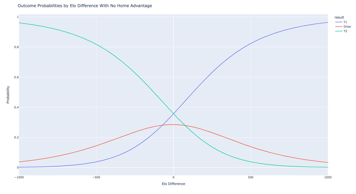
As expected, now the teams have the same odds when they have an Elo difference of 0.

But how does the model compare to actual results?

Since we are interested in measuring how accurate our probabilistic predictions are, we can’t use classic metrics such as F1 or Accuracy. Instead, we can create a calibration curve plot to measure how the model’s average prediction stacked against the observed win and draw rates. For the below curve, we fit the model to first ~5800 games, and then test the model on the remaining 3000 games.

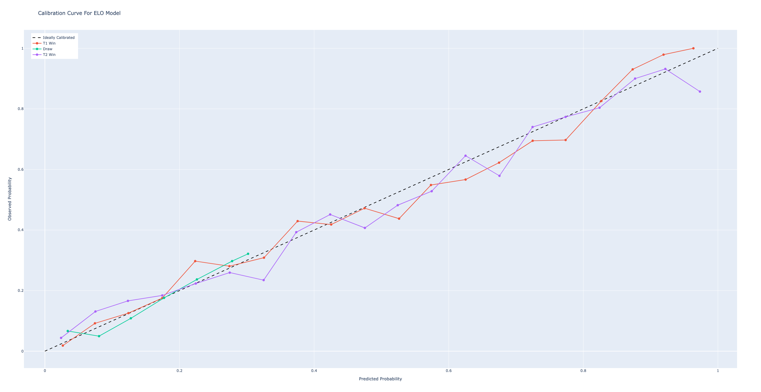
Generally, we can see the model’s probabilities track the true outcome, although there is some bias for some of the bins. To quantify the accuracy, we can calculate the model’s Expected Calibration Error (ECE), a weighted sum of each’s bin’s mean error. If you’re interested in learning more about the metric, I found this cool blog post that goes into more details and has nice visualizations. Our model has the following ECE values:

• T1 Win: 2.9%
• Draw: 1.6%
• T2 Win: 3.3%

Generally speaking, the model appears to be 3% off the observed results. However, to know how useful our model is, we should compare it to another international soccer model or betting odds. Unfortunately, I couldn’t find good historical international odds data, however we can compare our forecasts to Nate Silver’s prior 538 forecasts. For reference, here is the archived version of 538 methodology. The main metric we will use to evaluate the models’ efficacy is the famed Brier score, a metric to measure the performance of probabilistic forecasts.

Over 1510 games from 2019-03-23 and 2023-06-12, the 538 forecasts achieved a brier score of 0.518 whereas the ELO model presented in this post achieved a brier score of 0.512, suggesting both methodologies are comparable in accuracy. Not bad given the model’s simplicity!

Section 4: Remaining Thoughts

The first motivation of this post was to explain at a high level how I arrive at the international soccer forecasts published on this website. The second motivator was to show case that a (relatively) simple model can perform decently well and compete with other popular models (such as 538’s model).

Of course, I would be surprised if this model in a vacuum performs well with sports books or other betting exchanges, however it is a good starting point to build a more sophisticated model. My intuition is that international soccer matches are not priced as efficiently as domestic games because of the smaller sample sizes and higher variance (because of changing player form, team form, team availability, etc). Therefore, combining a simple (or more advanced) model with domain expertise could lead to more accurate betting odds.

As mentioned, this model is a starting point. Future directions to improve the model could (and probably should) include

1. Incorporating line up information and adjusting ELO based on relative squad strength
2. Acquiring more detailed match data (such as xG) to create a less noisy final score estimate to base the ELO ratings off of (similar to 538’s methodology)
3. Adjusting / fine tuning the ELO rating methodology
4. Incorporating other useful features into the regression such underlying performance metrics (attack and defense ratings), travel distance, or altidude

If you have any thoughts on the above, I would love to hear from you at mateojuliani at gmail dot com!