I learned about L2 / L1 regularization early on in my machine learning career as one of those empirical “tricks” one could use to prevent overfitting. The logic went as follows - by adding the sum of the squared (or absolute) value of the weights, you could prevent the model from learning large values for weights, which would prevent the network from learning weights that could perfectly model (overfit to) the data. Indeed, several blogs (such as this one by Google) provide a similar argument to the one above.

However, a lot of these blogs don’t mention why L2 regularization is the sum of weights squared, and not some other arbitrary function. The goal of this blog post is to discuss one derivation and interpretation of L2 / L1 regularization, and set the foundation for a research project I did for Columbia’s Probabilistic Models and Machine Learning course.

What is L2 regularization doing to the weights?

Although not explicitly mentioned, the Google post about regularization provides some hints at what L2 regularization is doing.

First, here is a chart from the blog post which shows the distribution of a model’s weight when using “low regularization”:

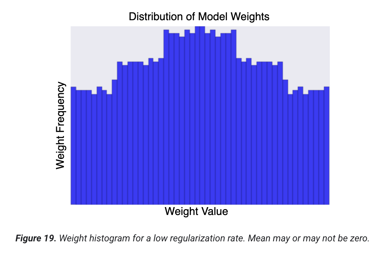
There seem to be some weights with higher values, some with lower values, but they all have some density. In contrast, here is the distribution of a model’s weight when using “high regularization” (i.e. L2 regularization):

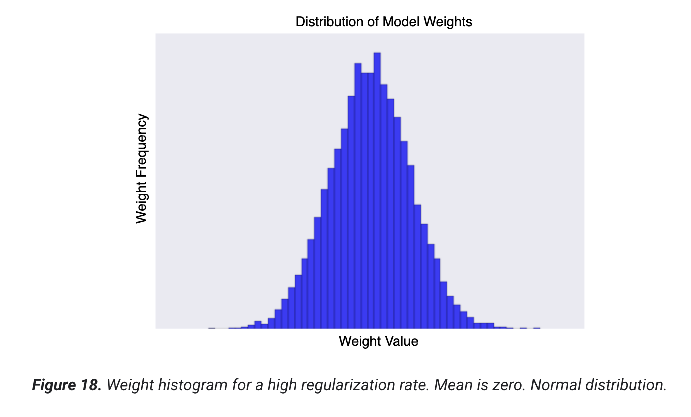
Woah! The distribution now resembles a normal distribution with mean zero. And there lies one interpretation of L2 regularization - L2 regularization assumes the values of each weight is sampled from a normal distribution with mean 0 and a fixed variance, $w_i \sim N(0, \lambda^2)$. Therefore, most of the weight values will be close to zero, given the probability of observing a large weight is low, but some higher valued weights will occur.

That’s pretty cool, but it still raises the question of where we get the $\sum_{i=1}^{n} w_i^2$.

Formal L2 Derivation

Bayesian Model Inference

To understand how we get the L2 derivation, we need to make a quick detour into Bayesian statistics. The core idea of Bayesian statistics is that you have a prior belief about something, you see some data (or evidence), and then you create a posterior belief based on the prior + the new data. We can apply the same concept to model inference. Suppose I have a dataset $D = {(x_i, y_i)}_1^n$ and I want to estimate a model’s parameters $\theta$. Under the Bayesian framework, I can estimate $p(\theta | D) \propto p(Y | \theta, X) p(\theta)$ using Bayes’ rules. In other words, my posterior model parameters are a function of the likelihood of me observing the data with parameters $\theta$ and data D ( the $p(Y | \theta, X)$) component times my prior belief on $\theta$ - $p(\theta)$.

Bayesian Regression Derivation

Okay, now lets see how one would actually implement this theory into practice.

First we need to define a model with our priors - in this case a multivariate linear regression model with a Gaussian prior. From a Bayesian modeling perspective, the target variable $y_i$ is sampled from $N(\beta \cdot x_i, \sigma^2)$, where $\sigma^2$ is fixed, and $\beta \sim N(0,\lambda^2)$. N denotes the normal distribution. For simplicity, we omit the intercept variable ¹.

To estimate the $\beta$, we will use the Maximum A Posteriori (MAP) estimate that seeks the single point that maximizes the posterior distribution of $\beta$ - $\arg \max_{\beta} \log P(\beta | \mathcal{D})$. In other words, we want to select the $\beta$ such that $N(\beta \cdot x_i, \sigma^2)$ best matches the distribution of the data D.

We can rewrite the posterior as $\beta_{MAP} = \arg \max_{\beta} [ \log P(\beta, \mathcal{D}) - \log P(\mathcal{D})]$. Since $P(\mathcal{D})$ doesn’t depend on $\beta$, we can ignore it and focus on the $P(\beta, \mathcal{D})$ portion of the maximization.

To maximize $\log P(\beta, \mathcal{D})$, we can use the product rule of probability to expand the joint distribution into the sum of our prior and the likelihood of the data:

$$\arg \max_{\beta} \log P(\beta, \mathcal{D}) = \arg \max_{\beta} \left[ \sum_{k=1}^P \log P(\beta_k) + \sum_{i=1}^n \log P(y_i | x_i, \beta) \right]$$

The right-hand term, $\sum_{i=1}^n \log P(y_i | x_i, \beta)$, is the standard Maximum Likelihood Estimate (MLE).

The left-hand term represents our prior belief about the weights. As mentioned earlier, we are assuming a Gaussian prior for our weights, meaning the probability density function is $P(\beta_k) = \frac{1}{\sqrt{2\pi}\lambda} e^{-\frac{\beta_k^2}{2\lambda^2}}$.

If we take the log of this Gaussian prior and drop the constant terms (since scaling constants don’t impact the location of the argmax), we are left with $-\frac{\beta_k^2}{2\lambda^2}$. Applying the same log-transformation to the Gaussian likelihood of our data gives us the standard squared error.

Plugging both of these back into our maximization equation yields our final form:

$$= -\frac{1}{2\lambda^2} \sum_{k=1}^P \beta_k^2 - \frac{1}{2\sigma^2} \sum_{i=1}^n (y_i - \beta \cdot x_i)^2$$

The term on the right is the negative of the standard linear loss function. On the left-hand side, we have an equation that looks very similar to the L2 regularizer (minimizing the sum of the squared weights), but with an extra term that involves $\lambda$. Typically, the constant in L2 regularization appears as a hyperparameter $\alpha$. In other words, this means that the choice of $\alpha$ specifies the Gaussian distribution. A larger $\alpha$ equates to a smaller $\lambda$, meaning that the weights will be closer to zero, which means heavier regularization.

And there we have it! L2 regularization is simply the result of assuming the prior distribution of your weights is gaussian!

But is L2 Regularization All We Need?

After reading this, a natural next question is - does a gaussian prior on the weights make sense for a neural net? Further, are there other priors that could lead to increased performance? This is the question I asked in this project.

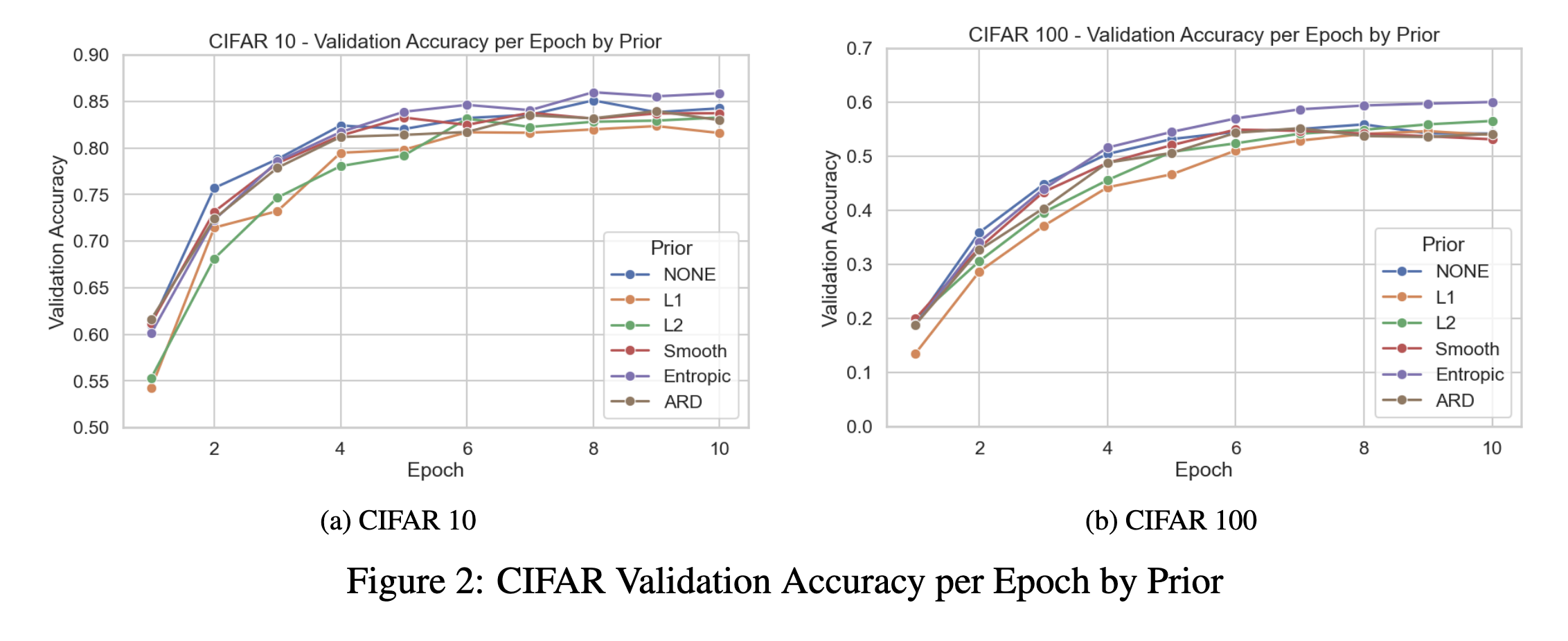
As a sneak peak, here is Figure 2 from the paper, providing the validation accuracy per epoch by the different priors (regularizors) for both the CIFAR 10 and CIFAR 100 datasets using a ResNet18-esque architecture. The Entropic prior is able to converge to a higher accuracy at a faster rate than the other priors.

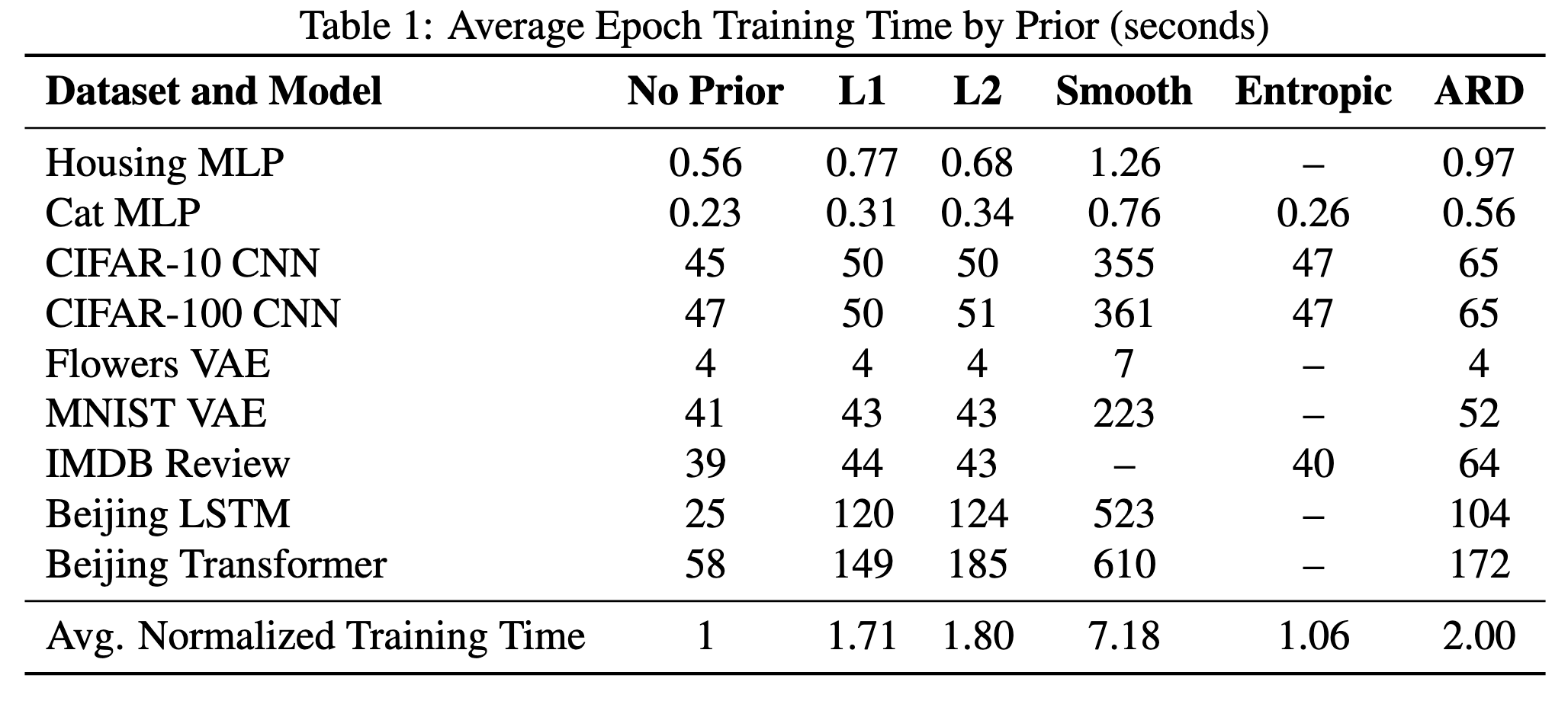
Interestingly, the entropic prior is also computationally cheaper than traditional L1 / L2 regularization, as show in table 1 of the paper:

The paper goes into further detail explaining the priors and experimental results, however we arrive to the following conclusion: maybe L2 regularization is not all we need (and maybe we should check out the entropic prior). Check it out!